# Multi-scale spiking network model of macaque visual cortex

This code implements the spiking network model of macaque visual cortex developed
at the Institute of Neuroscience and Medicine (INM-6), Research Center Jülich.
The model has been documented in the following publications:
1. Schmidt M, Bakker R, Hilgetag CC, Diesmann M & van Albada SJ
Multi-scale account of the network structure of macaque visual cortex
Brain Structure and Function (2018), 223:1409 [https://doi.org/10.1007/s00429-017-1554-4](https://doi.org/10.1007/s00429-017-1554-4)
2. Schuecker J, Schmidt M, van Albada SJ, Diesmann M & Helias M (2017)
Fundamental Activity Constraints Lead to Specific Interpretations of the Connectome.
PLOS Computational Biology, 13(2). [https://doi.org/10.1371/journal.pcbi.1005179](https://doi.org/10.1371/journal.pcbi.1005179)
3. Schmidt M, Bakker R, Shen K, Bezgin B, Diesmann M & van Albada SJ (2018)
A multi-scale layer-resolved spiking network model of
resting-state dynamics in macaque cortex. (under review)
The code in this repository is self-contained and allows one to
reproduce the results of all three papers.
## Python framework for the multi-area model
[](https://www.python.org) <a href="http://www.nest-simulator.org"> <img src="https://raw.githubusercontent.com/nest/nest-simulator/master/extras/logos/nest-simulated.png" alt="NEST simulated" width="50"/></a>
The entire framework is summarized in the figure below:
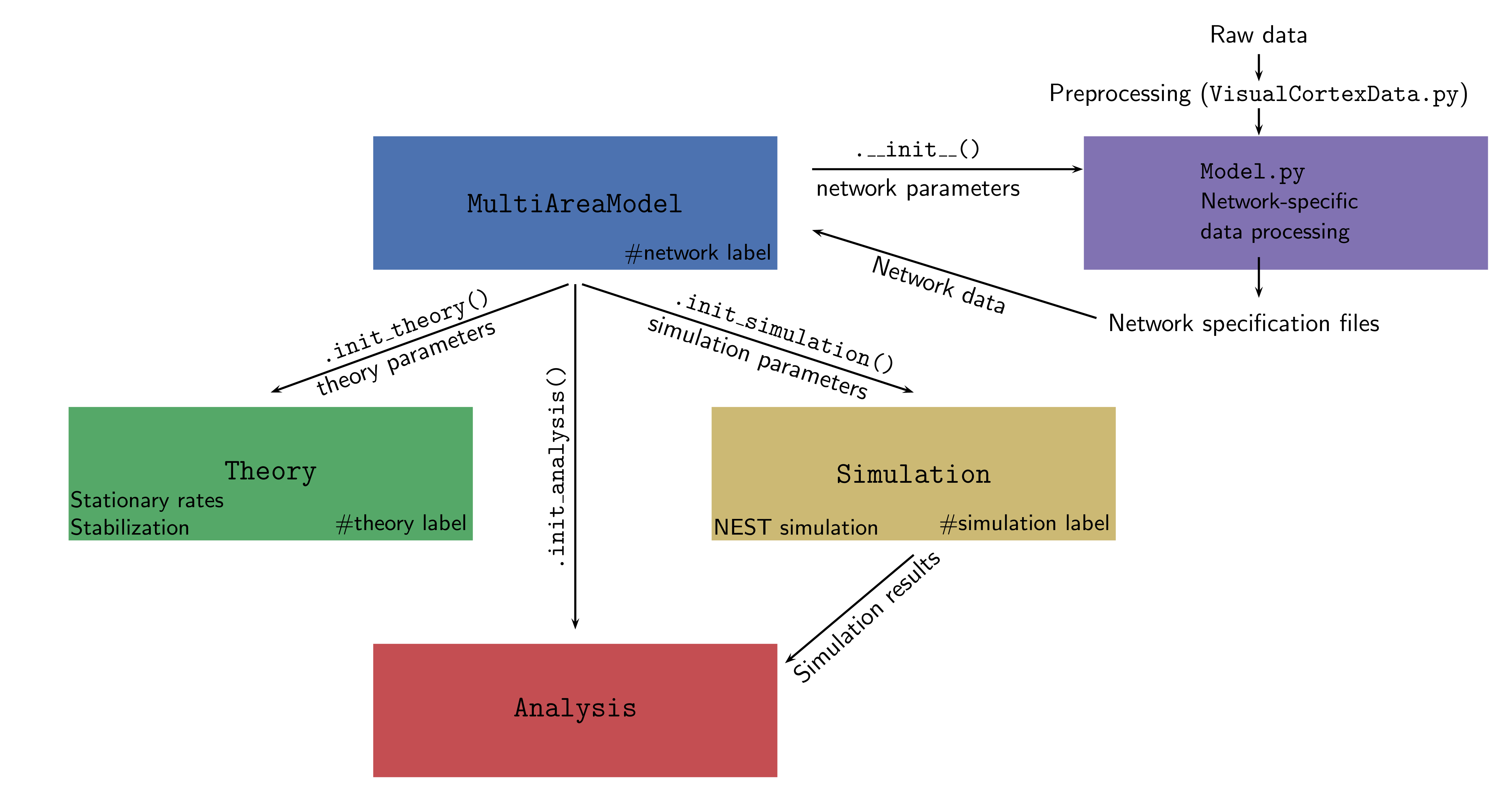
In principle, we strictly separate the structure of the network
(defined by population sizes, synapse numbers/indegrees etc.) from its dynamics
(neuron model, neuron parameters, strength of external
input, etc.). The complete set of default parameters for all components
of the framework is defined in `default_params.py`.
--------------------------------------------------------------------------------
To start using the framework, the user has to define a few environment variables
in a new file called `config.py`. The file `config_template.py` lists the required
environment variables that need to specified by the user.
Furthermore, please add the path to the repository to your PYTHONPATH:
`export PYTHONPATH=/path/to/repository/:$PYTHONPATH`.
--------------------------------------------------------------------------------
`MultiAreaModel`
The central class that initializes the network and contains all
information about population sizes and network connectivity. This
enables reproducing all figures in [1]. Network parameters only
refer to the structure of the network and ignore any information on
its dynamical simulation or description via analytical theory.
`Simulation`
This class can be initialized by `MultiAreaModel` or as standalone and
takes simulation parameters as input. These parameters include, e.g.,
neuron and synapses parameters, the simulated biological time and also
technical parameters such as the number of parallel MPI processes and
threads. The simulation uses the network simulator NEST
(https://www.nest-simulator.org). For the simulations in [2, 3], we
used NEST version 2.8.0. The code in this repository runs with a
later release of NEST, version 2.14.0 .
`Theory`
This class can be initialized by `MultiAreaModel` or as standalone and
takes simulation parameters as input. It provides two main features:
- predict the stable fixed point of the system using mean-field theory
- execute the stabilization method described in [2] on a network instance (will be provided soon)
`Analysis`
This class allows the user to load simulation data and perform some
basic analysis and plotting.
## Analysis and figure scripts for [1-3]
The `figures` folder contains a subfolder with all scripts necessary to produce
the figures from [1]. The scripts for [2] and [3] will follow soon.
If snakemake is installed, the figures can be produced by executing
`snakemake` in the respective folder:
cd figures/Schmidt2018/
snakemake
## Running a simulation
A simple simulation can be run in the following way:
1. Define custom parameters
custom_params = ...
custom_simulation_params = ...
2. Instantiate the model class together with a simulation class instance.
M = MultiAreaModel(custom_params, simulation=True, sim_spec=custom_simulation_params)
3. Start the simulation.
M.simulation.simulate()
Typically, a simulation of the model will be run in parallel on a compute cluster.
The files `start_jobs.py` and `run_simulation.py` provide the necessary framework
for doing this in an automated fashion.
The procedure is similar to a simple simulation:
1. Define custom parameters
custom_params = ...
custom_simulation_params = ...
2. Instantiate the model class together with a simulation class instance.
M = MultiAreaModel(custom_params, simulation=True, sim_spec=custom_simulation_params)
3. Start the simulation.
Call `start_job` to create a job file using the `jobscript_template` from the configuration file
and submit it to the queue with the user-defined `submit_cmd`.
The file `run_example.py` provides an example.
Be aware that, depending on the chosen parameters and initial conditions, the network can enter a high-activity state, which slows down the simulation drastically and can cost a significant amount of computing resources.
## Simulation modes
The multi-area model can be run in different modes.
1. Full model
Simulating the entire networks with all 32 areas and the connections between
them is the default mode configure in `default_params.py`.
2. Down-scaled model
Since simulating the entire network with approx. 4.13 million neurons and 24.2 billion
synapses requires a large amount of resources, the user has the option to scale down
the network in terms of neuron numbers and synaptic indegrees (number of synapses
per receiving neuron).
This can be achieved by setting the parameters `N_scaling` and `K_scaling` in `network_params`
to values smaller than 1. In general, this will affect the dynamics of the network.
To approximately preserve the population-averaged spike rates, one can specify a set of target rates
that is used to scale synaptic weights and apply an additional external DC current.
3. Subset of the network
You can choose to simulate a subset of the 32 areas specified by the `areas_simulated`
parameter in the `sim_params`. If a subset of areas is simulated, one has different options for how to replace the rest of the network set by the `replace_non_simulated_areas` parameter:
- `hom_poisson_stat`: all non-simulated areas are replaced by Poissonian spike trains with the
same rate as the stationary background input (`rate_ext` in `input_params`).
- `het_poisson_stat`: all non-simulated areas are replaced by Poissonian spike trains with
population-specific stationary rate stored in an external file.
- `current_nonstat`: all non-simulated areas are replaced by stepwise constant currents with
population-specific, time-varying time series defined in an external file.
4. Cortico-cortical connections replaced
In addition, it is possible to replace the cortico-cortical connections between simulated
areas with the options `het_poisson_stat` or `current_nonstat`.
## Testsuite
The `tests/` folder holds a testsuite that tests different aspects of network model initalization and meanfield calculations.
It can be conveniently run by executing `pytest` in the `tests/` folder:
cd tests/
pytest
## Requirements
python\_dicthash ([https://github.com/INM-6/python-dicthash](https://github.com/INM-6/python-dicthash)),
correlation\_toolbox ([https://github.com/INM-6/correlation-toolbox](https://github.com/INM-6/correlation-toolbox)),
pandas, numpy, nested_dict, matplotlib (2.1.2), scipy, NEST 2.14.0
Optional: seaborn, Sumatra
To install the required packages in a conda environment, execute:
`conda env create -f environment.yaml`
Note that NEST needs to be installed separately, see <http://www.nest-simulator.org/installation/>.
In addition, reproducing the figures of [1] requires networkx, python-igraph and pyx. To install these additional packages, execute:
`pip install -r figures/Schmidt2018/additional_requirements.txt`
In addition, Figure 7 of [1] requires installing the `infomap` package to perform the map equation clustering. See <http://www.mapequation.org/code.html> for all necessary information.
The SLN fit in `multiarea_model/data_multiarea/VisualCortex_Data.py` and `figures/Schmidt2018/Fig5_cc_laminar_pattern.py` is currently not possible because of copyright issues.
## Contributors
All authors of the publications [1-3] made contributions to the scientific content.
The code base was written by Maximilian Schmidt, Jannis Schuecker, and Sacha van Albada. Testing and review was supported by Alexander van Meegen.
## Citation
If you use this code, we ask you to cite the appropriate papers in your publication. For the multi-area model itself, please cite [1] and [3]. If you use the mean-field theory or the stabilization method, please cite [2] in addition. We provide bibtex entries in `CITATION`.
<img src="https://raw.githubusercontent.com/nest/nest-simulator/master/extras/logos/nest-simulated.png" alt="NEST simulated" width="200"/>